NCSA wiki will be offline Friday, Apr 19, 2024, from 1700 hours until Sun, Apr 21, 2024 in order to upgrade Confluence.
MAEviz Overview
Welcome 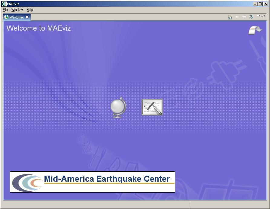
When MAEviz is first launched, the welcome screen appears. From the welcome screen, users can select to read an overview of information about MAEviz, follow built-in tutorials, or just begin working in MAEviz (by selecting Workbench which will take you to the main MAEviz screen, also known as the Workbench). See figure above.
Workbench Layout
The MAEviz workbench consists of a number of Views, each containing information about a specific part of MAEviz. Each view is like a sub-window within the MAEviz workbench window, and can be minimized, maximized, moved, or even torn away from the main window into its own window. These interactions are done by clicking the minimize and maximize view icons in the view's title bar, or by clicking and dragging on the view's border or title bar.
See the image below for the most commonly used views in MAEviz.
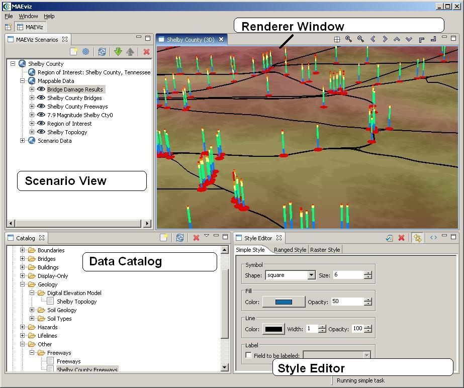
Scenario View
The Scenario View is where you will find a list of all the data for the scenario or scenarios that you are currently working with. Each scenario that you are working with is listed as a top-level item in this view, which can be expanded by clicking the plus ![]() icon next to its name, to see the details of the scenario. Inside each scenario, you can see a list of the Mappable Data and Scenario Data. All data listed in Mappable Data are the layers of data that appear in your rendered map whereas all the data listed in the Scenario Data includes all non-renderable data for the scenario (e.g. tables).
icon next to its name, to see the details of the scenario. Inside each scenario, you can see a list of the Mappable Data and Scenario Data. All data listed in Mappable Data are the layers of data that appear in your rendered map whereas all the data listed in the Scenario Data includes all non-renderable data for the scenario (e.g. tables).
The Scenario View is also where you would go to do the major operations on your scenarios: adding an earthquake hazard or other data, running damage analyses, etc.
Visualization View
The Visualization Window Views are where the rendered maps of your scenario will appear. Each scenario can have its own rendered 2d and 3d map, so you can see the visualization multiple scenarios simultaneously if desired. It is here that you can get a quick visual overview of the results of your analyses. You can control the camera position by using the mouse, or click the view control buttons in the toolbar.
Data Catalog View
The Catalog View is a list of all the data that is available for you to use in your scenarios. It is organized first by repositories, which are stores of MAEviz data. Repositories can represent local data, or data stored on a remote server. Within each repository, the data is organized by the type of data that it is. To add data to a scenario, you can navigate to and find the data within this view, then drag it into either the Visualization View for your scenario, or onto the scenario's name in the Scenario View. Before data can be made available to your scenario, it must be ingested into a repository and assigned a type. You can find instructions on ingesting building data here.
Style Editor View
The Style Editor is used to adjust the way in which a layer of data is displayed in the Visualization View. If the Style Editor is not visible, you can show it by right clicking a Mappable Data layer in the Scenario View, and selecting Change Layer Style. Once this view is showing, you can adjust the color, shape, opacity, and other display characteristics of the map layer. To apply your style changes, you must click the Apply button (  ) in the view's toolbar.
Other Views
Although these are some of the main views you will use, there are a few other views that are shown at various times while using MAEviz and we'll discuss them below.
Table View
The Table View is used to display tabular data such as the attributes of a set of inventory data or analysis results. The most common way to see this view is by right-clicking a Mappable Data layer in the Scenarios View and selecting Show Attribute Table.
Reports View
By right-clicking on a scenario name in the Scenarios View, and selecting Reports..., you can access the Select Report View. By default there are two report types available for every result based on the metadata for each result type, the Default Summary Report and Default Detail Report. The summary report will provide a summary of results and the detail report will provide explicit detail about each result (e.g. building by building results). To run a report, select the report you wish to run, right-click on it and select the Run Report option. The selected report will be generated and displayed. From that point, you can choose to print or save the report.
Fragility View
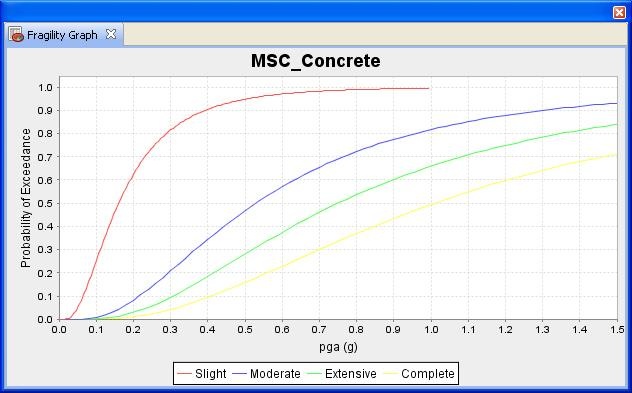
If you right-click a fragility dataset from the Catalog View, you can select View Fragility to access the Fragility View. The Fragility View shows a list of fragility types that you can drill down into to select and view a particular fragility curve. When you have found the fragility curve that you want to view, right-click it and select View Fragility Set to view a graph of the fragility curve. See the image below.
MAEviz Tutorial
Example Scenario
In this demonstration, we will use MAEviz as a specific stakeholder would use the tool. Consider the stakeholder to be an Emergency Manager who wishes to determine possible impacts of earthquake hazards on Shelby County Tennessee buildings. The Emergency Manager wishes to investigate the impact of a specific speculated earthquake on the existing building stock in Memphis and Shelby County Tennessee. Consider this analysis to be preliminary, and therefore limit the scope of the study by neglecting single family residences. For this analysis we will use a fictitious moment magnitude 7.7 event located at Marked Tree Arkansas.
In the process, we will see how the Emergency Manager will launch the MAEviz application, load the GIS data for Shelby County, and then generate earthquake hazard information based on the scenario he wants to investigate. After he has loaded this base information, he can interactively choose and display information for the specific items he wants to evaluate - the buildings, as well as load fragility information for these particular structures. From there, we will witness an analysis of the impact of the hazard. These factors have important social and economic impacts which can be investigated with more advanced analyses that MAEviz has available.
Creating a New Scenario
- When you start MAEviz and if this is the first time you have run MAEviz, you will be shown the welcome screen. To begin working with MAEviz, click the rightmost icon (
 ) which will take you directly to the MAEviz workbench.
 - From the application's menu bar, click File -> New Scenario. Alternatively, you can click the New Scenario button (
 ) from the Scenario View's tool bar
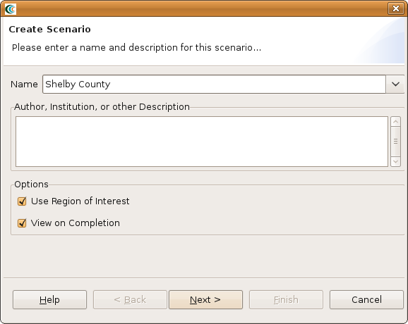
 - The New Scenario Wizard will now be showing. This is where you define the scenario that you would like to work with. Enter a name for your scenario, such as "Shelby County", and then optionally enter any descriptive information about the scenario in the large text box. Click the Next button. See the figure below.
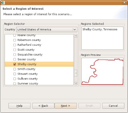
- At this point, you will be selecting the region of interest that you would like to work with. We will be analyzing Shelby County, TN, so select United States of America from the Country menu. You should see a list of states appear in alphabetical order. Scroll down to find the state of Tennessee and click the
 symbol next to Tennessee. You will now see a list of counties displayed. Scroll down to find Shelby County and click the box so that a check appears next to the name. You should now see Shelby County, Tennessee populate the Regions Selected box. This new region of interest wizard allows you to add multiple regions of interest by checking other boxes of regions you want to use; however, for this tutorial we will only focus on Shelby County (See figure below). Click Next when finished.
- The next screen allows you to select a default set. This will populate the analysis user interface pages with default data where applicable (e.g. default fragilities, default fragility mapping, etc). From the dropdown menu, select "MAEviz 3.0 Shelby County Analysis Defaults". Note: For completeness, this tutorial will assume that no default set has been chosen so you might find some fields that you are requested to fill in already filled in for you. In these cases, you can ignore the tutorial instructions. Click Finish to complete the wizard and have MAEviz initialize your new scenario
Viewing the Scenario and Adding Data
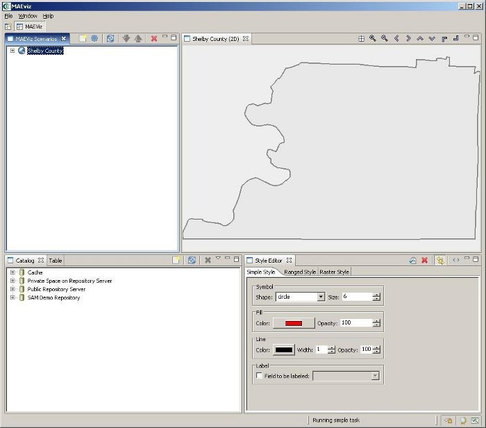
At this point, your scenario has been created. You will see your scenario listed in the Scenario View and a blank outline of Shelby County has appeared in the Visualization View. See figure below.
Next, we will learn how to add data to our scenario, and how to manipulate the Visualization View.
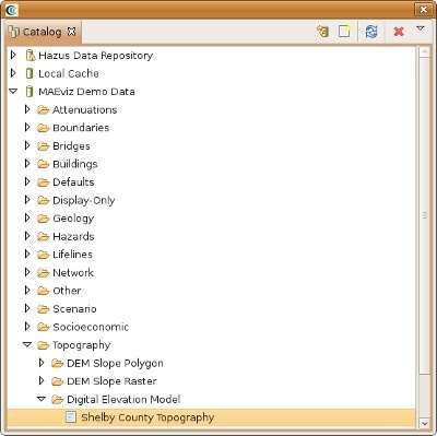
First, we will add elevation data to the scenario. In the Catalog view (the lower-left view of your workbench is arranged in the default setting, as shown in the figure below), expand the MAEviz Demo Data item, then Topography and finally Digital Elevation Model. Click and drag the Shelby County Topography item into the Visualization View.
At this point, an elevation map should have been added to the Visualization View. We will also add building information to the Scenario. Under the Catalog View, still under the MAEviz Demo Data item, expand Buildings, then Building Inventory v5.0, then Shelby County No SF Buildings v5. Drag the dataset for Shelby County No SF Buildings v5, which excludes single family homes, into the Visualization View as well. Alternatively, you can right-click the item and select Load Dataset.
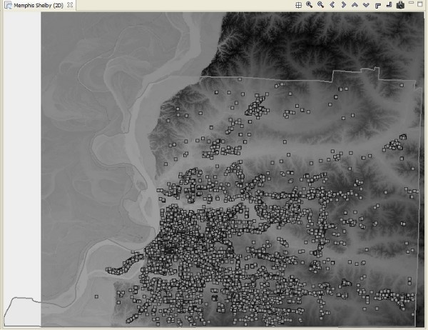
At this point, your Visualization View should look similar to the image below:
To make the buildings easier to see, we will adjust their map style. From the Scenario View, expand Shelby County, then Mappable Data. You should see the list of the data that you added to the Scenario. Right click on Shelby County No SF Buildings v5, and choose Change Layer Style.
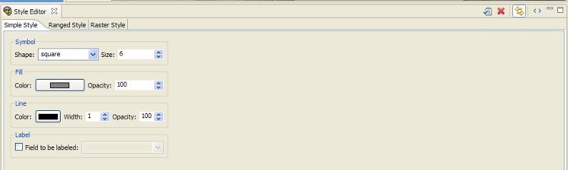
In the Style Editor (see figure below), the Simple Style tab should be active. Click the black box labeled Color, and select a color that is easier to see, such as yellow. Click Ok in the color selection box and then to apply the style change, click the Apply Style button in the Style Editor's tab bar. ( )
Some visualization controls:
- To zoom/pan/etc, use the controls at the top of the Visualization View. Use these to adjust your view.
- To view a 3d rendered view of the same information, right click the entry for your Scenario, and choose Render in 3D (VTK). This will bring up a second Visualization View that shows the same map, but from a 3d rendered perspective.
- After adjusting your view, if you want to restore to the original default view in the Visualization, click the Zoom to full extent button in the toolbar (
 )
)
Running an Analysis
Now that we have a basic map to look at, we will learn how to run an analysis. Analyses in MAEviz consist of any sort of calculation that generates data. For example, generating a deterministic earthquake map based on a magnitude and epicenter would be considered one type of analysis. Using that earthquake map as well as building inventory data to generate information about building damage would be another type of analysis.
In this example, we want to find building damage results based on a deterministic earthquake hazard that we will specify.
- First, we will launch the Run Analysis Wizard. To do so, you can click the Execute Analysis toolbar button (
 ).
). - This causes the Run Analysis Wizard to be shown. See figure below. Here you can select which analysis you want to run. From this page, expand Building, and select the Structural Damage analysis. Click Finish.

- The page that displays will show you a graphical view of the damage analysis, including all of its inputs and the current readiness of the analysis. See the figure below.
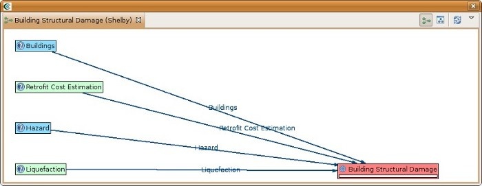
- The red background of Building Structural Damage indicates that not all required inputs have been set. To begin, click once on the Building Structural Damage box and an input form should appear below the analysis graph. See figure below. Under the required tab of the form, you will need to provide several inputs. Looking at the blank form, it tells you that no datasets containing Fragilities, Expected Value or Fragility Mapping have yet been loaded into your scenario. To run this analysis, you must load datasets that contain these data.

- To help you locate or generate the necessary input data, the Analysis Form provides two types of buttons, the Find Dataset button (
 Search), and the Create Dataset from Analysis button ( Create)
- To find a Fragilities dataset to run your building damage with, click the Find Dataset button ( ). The window that appears contains a list box of all Fragilities Datasets that could be found in any of the data repositories that you are connected to. Select Default Building Fragilities 1.0 from the list, and click Finish. See the figure below. To find an Expected Value dataset follow the same steps for the related field and select Building Damage Ratios v1.1 from the list, and click Finish. Follow the same steps for the Fragility Mapping dataset but select Default Building Fragility Mapping 1.0 from the list.

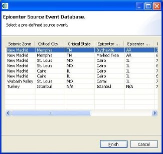
- For our hazard, we want to create a deterministic earthquake hazard. So this time, use the Create button to add a scenario earthquake analysis node to the graph. Click on the Create Scenario Earthquake box and you should see a form similar to the structural damage analysis form. You will need to fill in a result name and select CEUS Characteristic event for the Attenuation. Under Earthquake Location, click on the link that says Select from Source Event. From the dialog box that appears, select the first event in the list and click Finish. See figure below.
- After doing this, both the Create Scenario Earthquake box and the Building Structural Damage box should have turned green. Click the Execute button
- Alternatively, we could have clicked the optional tab on the structural damage analysis form and selected to apply some retrofits. By default, MAEviz will use the as-built fragility for each building.
- Once the progress bars have finished for each analysis, you should see new datasets added to your Scenario View and map: The Building Inventory v5 dataset that you selected to use, a Building Damages dataset which will contain the damage information, and the earthquake hazard dataset. Your Visualization should now look similar to the figure below with the buildings colored by mean damage.

- To change the visualization for this dataset, right click on the Building Damage layer, and select Change Layer Style. The Style Editor should appear in the bottom right of the application window. Like other windows, you can move or resize it to make it easier to view. Select MeanDamage or another field from the drop down menu as the Value in the Field Classified section. After picking the field to view, select the Number of Classes to classify (e.g. mean damage) on buildings. To apply the style change, click the Apply Style button in the Style Editor's tab bar. ( )
- Before looking at the economic impact of this scenario, we should first compute the non-structural and content damage. To do this, go back to the Execute Analysis button ( ) and select the Non-Structural Content Damage (generalized) and click Finish. As before, click on the analysis in the graph to open the input form. The new window shows parameters for creating the Building Non-Structural Content Damage like the figure below, based on the analysis you are executing, you should select the fragility mapping from the related field, and click Execute. Note: you should use the hazard we created in the building structural damage analysis for the non-structural damage.

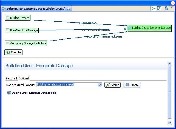
- Then, to see the economic impact, go back to the Execute Analysis button ( ) and select Direct Economic Damage and click Finish. You should see a page similar to the one in the figure below. The Non Structural Damage dataset is not a required input for the direct economic damage so you will need to select the optional tab to find that input field and select the non-structural dataset we just created. For the occupancy mapping, you should use the find dataset button, and click Execute to create the Building Direct Economic Damage. Note: Including structural and non-structural damage can make the direct economic damage calculation take a considerable amount of time to run so to improve running time, you can just include the structural damage.
- Now that we have the economic losses for the buildings, we can determine the fiscal impact of the economic loss. To do this, click the Execute Analysis button ( ) again and select the Fiscal Impact Analysis under the Socioeconomic category and click Finish. The new window shows the parameters for computing the fiscal impact (see figure below). The tax rate field is the default property tax rate to use for the region if no property tax map is provided. One optional field is to use a tax map; however, if one is available it will first need to be added to MAEviz by ingesting it. For this tutorial, we will ignore this field. Another optional field, Select Minimum DED, allows you to enter the minimum economic loss criteria used to select the buildings for inclusion in the property tax loss calculation. For example, entering 10.0 will only calculate the property tax loss for buildings that lost more than 10% of their value from direct economic damage. Those with less will be given the value 0 for property tax loss. Entering 0 for the field will include all buildings in the calculation, regardless of the amount of building value loss. For this analysis, we will include all buildings, which is the default operation. Click finish to generate the fiscal impact.

Decision Support
In this section we are going to illustrate how to run the Building Decision Support analyses in MAEviz. The analyses include the Building Decision Support Attributes Analysis, the Equivalent Cost Analysis(ECA), the Multi-Attribute Utility Analysis(MAUT) and the Individual Utility Analysis. The Building Decision Support analysis computes the decision attributes such as monetary loss, injuries, deaths and function loss that can be used by the Equivalent Cost Analysis to turn the non monetary attributes into monetary attributes for making decisions. Alternatively, these attributes can be given to the Multi-Attribute Utility Analysis to compute the overall utility of the results. The Individual Utility Analysis provides the change in utility for retrofitting a single structure while leaving all other structures unchanged. This is useful for determining which building(s) give the best return for your investment.
Before going through the decision support process, there are a few things the user will need to get the most out of these analyses. For the equivalent cost analysis, the user will need conversion values for the non-monetary variables such as injuries, deaths and days of function loss or use the pre-defined values in MAEviz. For the multi attribute utility analysis and the individual utility analysis, the user will need to define utility curves for each attribute as well as determine what the weight of each attribute is in the overall utility. Example curves are available, but will not provide good results because they are not defined to work with the dataset we have and were meant only for illustration purposes.
Decision Attributes
Let's use the building dataset we already have loaded to generate some decision attributes that we can then use in the ECA and MAUT analysis. We can choose to either use the damage datasets we have already generated or generate some new datasets. For now, we'll use what we already have since we will need to obtain the as-built decision attributes to find the incremental change in utility for upgrading structures one at a time.
- First, we will need to launch the Run Analysis Wizard again. To do so, you can click the Execute Analysis toolbar button ( ). Find the Decision Support category and expand it. Select Building Decision Support Attributes and click Finish.
- Click on the Building Decision Support Attributes icon in the graph to bring up the form page. For Result Name, specify As-built Decision Support Attributes, for Structural Damage, select the structural damage dataset you created previously, for Non-Structural Damage, select the previously created non-structural damage dataset, for Retrofit Cost Estimate, click the Create button and specify something like Building Retrofits for the Result Name field and for the Buildings field, select our building dataset. Click on the Building Decision Support Attributes icon again and scroll down until you find the Population Estimate Type field and specify Crude Population Estimate. This will use a very simple calculation of time of day and square footage of the building to estimate population. For the Decision Attributes, the default values are fine.
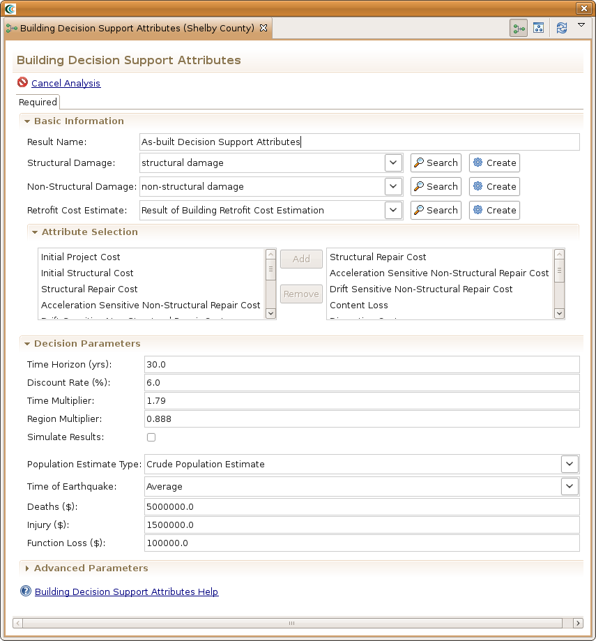
- A few more things to note about this analysis. You can check the Simulate Results box to perform a Monte-Carlo simulation over the specified number of simulations. Also, you can adjust the values specified for the injuries, deaths, and functional loss as well as time of day of the event, the discount rate, the time horizon, etc. All fields you see can be tweaked, but the user should only do this if they feel comfortable tweaking the values.
- After making any final adjustments, click the Execute button to run the analyses.
Equivalent Cost Analysis
Now that we have the as-built decision attributes, let's run the Equivalent Cost Analysis to assign the decision variables dollar values so we have a common unit that can be added to obtain total loss.
- Bring up the Run Analysis Wizard again and expand the Decision Support category and select Equivalent Cost Analysis. Click the Finish button.
- Click on the Equivalent Cost Analysis box in the analysis graph to bring up the form page.
- For Result Name, choose something like As-Built ECA and for Building Decision Support Attributes, choose the dataset you just created in the previous step. In the Decision Parameters section, you can either choose to change the conversion values for the non-monetary variables or leave the defaults.
- Click the Execute button.
- You should now have a new dataset with the monetary cost of each decision variable for each building.
One useful visualization for these results is running a statistical analysis on the results. Do the following to bring up the statistics view.
- Right click on the new dataset (e.g. As-Built ECA), and select Show Attribute Table. This should bring up the Table View of the results. In the Table View, find and click on the summation (
 ) icon. You should see something similar to the
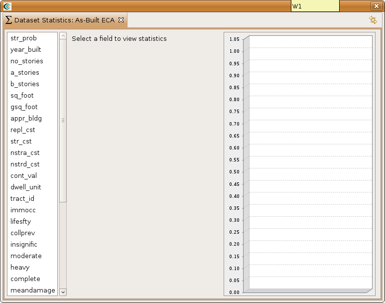
- To generate statistics for a particular field, click on it in the left hand box. For example, scroll down and find the injury_m field and click on it. That is the total injuries converted to a monetary value. You should now have something similar to the image below.
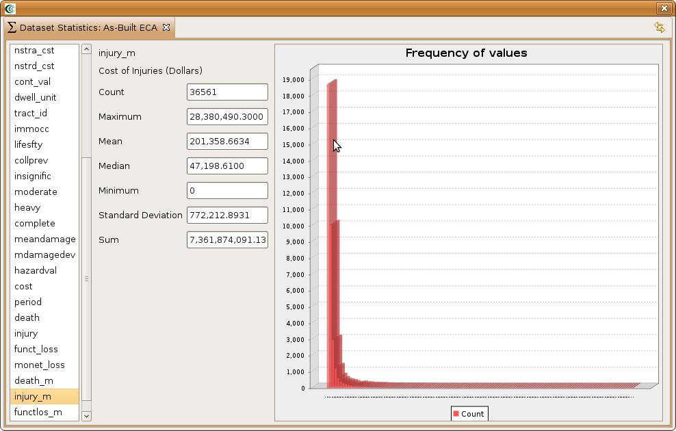
- For the injuries_m field we can see the Count, Maximum, Mean, Median, Minimum, Standard Deviation, and Sum. For this field, the more important values are the Sum, which tells use the overall total cost of the injuries from the earthquake, the Maximum, which tells us what the highest cost from injuries was, and the Mean value of injuries for each building. If the Maximum value is large, then we might just need to focus on a few structures to minimize injuries and potential loss of life.
Multi-Attribute Utility Analysis
Perhaps more informative than the Equivalent Cost Analysis is the Multi-Attribute Utility Analysis (MAUT). Instead of converting the non-monetary decision variables to monetary values as the common unit for addition, we convert the decision variables to utility values. Each decision variable is given a weight so that the overall utility adds to at most, 1.0. This can be very useful since assigning value to life can be difficult and can better be measured by acceptable and unacceptable consequences. The user also has more control over how each variable weighs into the overall utility. For example, maybe injury and death prevention are most important and monetary cost is least important. The decision maker can give more weight to the death/injury utilities so that if deaths and injuries are minimized, a higher utility value will be obtained thus allowing us to better judge the retrofit strategy.
This also makes it more clear why a decision maker must define their own utility curves. Every decision maker will have a different view on what are acceptable and unacceptable consequences. It is important for decision makers to define utility curves that describe their risk attitude so that the decision support tools can provide the best possible guidance. That being said, below we will outline how to use the sample utility functions that will illustrate how MAUT works.
- Bring up the Run Analysis Wizard again and expand the Decision Support category and select Multi-Attribute Utility Analysis. Click the Finish button. When the analysis graph is displayed, click on the Multi-Attribute Utility Analysis block in the graph and you should see a view similar to the one below.

- On the form page there are several fields that need to be filled out. For the Result Name field, specify something like As-Built MAUT. If you are using version 3.1.1 or earlier, then for the MAUT Results field select As-built Decision Attributes. Otherwise, you should see a field called Building Decision Support Attributes and you should select As-built Decision Attributes for that field.
- By default, the Risk Attitude is set to Risk Averse and the Variable Weights are User Defined. If you select MAEviz Calculated, then MAEviz will calculate the weights based converting the maximum values for each decision variable into dollar amounts and dividing by the total dollar amount for all variables. (e.g. (deaths x monetary-conversion) / (total dollars for all weights)). In the Advanced Parameters section, users can select a utility curve dataset. The default is eScience Sample Utility Functions, which were generated for an e-Science demonstration of MAEviz.
- After making the desired changes, click the Execute button.
- When the analysis has finished, there should be a new dataset with the name you provided in your scenario. If you right click on the dataset and select Show Attribute Table, you will see there is a new column called utility that has been added. This is the overall utility for the entire dataset. In our case, the utility is zero, which we could have guessed from looking at the utility functions and the results we had in our Building Decision Support Attributes dataset. The acceptable deaths limit was 30 and the acceptable injury limit was defined at 55, these numbers are well below what our expected death and injury totals, thus the very low utility score. The utility curves were defined for a small dataset and not intended for such a large dataset as ours.
Individual Utility Analysis
The last analysis for decision support that we want to illustrate is the Individual Utility Analysis. We already have the as-built damage so all we need to do is generate another damage dataset with building upgrades and its associated Building Decision Support Attributes dataset.
- Bring up the Run Analysis Wizard again and expand the Decision Support category and select Individual Utility Analysis. Click the Finish button. When the analysis graph is displayed, click on the Individual Utility Analysis block in the graph and you should see the form page appear.
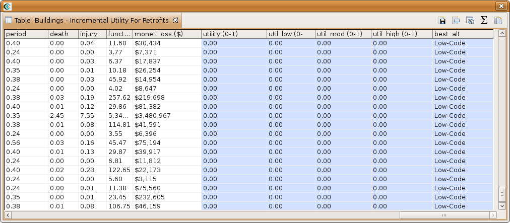
- Some of the data we have already so we can fill that in. For Result Name, I suggest using something like Buildings - Incremental Utility For Retrofits.
- For the As-Built Decision Attributes field, select the dataset we already created from the drop down menu.
- You will notice that the Upgraded Decision Attributes Results field allows multiple inputs. This is because users might want to create a dataset with all low-code upgrades, all moderate-code upgrades and all high-code upgrades to see which upgrade gives the best return on investment. There might be a minor difference between as-built and low-code, but a more significant difference when upgrade to moderate-code. This would not be obvious unless you do all retrofit levels. For simplicity, we will only do a single upgrade to low-code since the user would only need to repeat the process we outline in the next few steps.
- Click on the Create button ( ) next to the Upgraded Decision Attributes Results field. This will add a Building Decision Support Attributes box to the graph view. Click on it to bring up its form page.
- For Result Name, use something like Low-Code Decision Attributes, for the non-structural damage, we can re-use the previously created non-structural damage because reinforcing the structure does not effect the non-structural damage. We can also select the previous retrofit cost estimation dataset. For the Attribute Selection, select the same attributes as you did for the as-built decision attributes so we have homogeneous datasets. For the population estimate, choose the same as previous (in our case we chose the Crude Population Estimate). If you made any other changes for the as-built decision attributes, make the same selections again. Finally, we need the new building damage after low-code upgrade so click on the Create button ( ) next to the Structural Damage field and click on the Building Structural Damage box to bring up the form page.
- For the Result Name field, choose something like Low-Code Structural Damage. For the Buildings field, choose the previously loaded building dataset. For the Hazard field, click on the Search button ( ) and locate the scenario earthquake we already created.
- Next, click on the Optional tab. In the Retrofit Cost Estimation field, choose the previously created retrofit cost dataset. This should populate a new field. Click on the Select Retrofits and select setAllTo. This should bring up a dialog box with the available retrofits, select Low Code Retrofit and click OK. Note: only the buildings with low-code available as a retrofit will be changed in the form page. Some buildings either don't have a low code retrofit fragility or are already considered low-code buildings. In these cases, the as-built fragility will be used so there will be no change in utility.
- At this point the analysis is ready to go. If you made any other changes to any of the form pages when computing the as-built decision support attributes, make sure those same selections have been made now so that we have homogeneous datasets. Click the Execute button. It may take some time to finish this analysis depending on the size of your dataset since each building is being changed one at a time to see the change in utility.
After the analysis finishes, you will have 5 additional columns. The utility column has the as-built utility value for the non-retrofit scheme. Following that are 3 columns, util_low, util_mod and util_high, which gives the change in utility if the building is upgraded to low code, to moderate code and to high code. The last column lists the best alternative based on the 3 utility values. For this to be useful we would have needed to do decision support attributes for moderate code and high code. You should see an attribute table similar to the one below if you used the settings we did
Analyzing Results
Now that the analyses that we were interested in have been completed, it's time to analyze and try to make sense of the results. There are various ways of viewing and visualizing the results, which we will learn now.
Table View Results
- First, we will view the results in a tabular grid, similar to an MS Excel spreadsheet. In the Scenario View, right click on the structural damage layer, and select Show Attribute Table. The Table View should appear in the bottom right of the application window. Like other windows, you can move or resize it to make it easier to view.
- Now we will use the Table View to locate the buildings that suffered the most damage. Scroll to the right edge of the table view, and click the column header labeled MeanDamage, which is the column containing the mean damage value for each building. This will sort the table by the mean damage value.
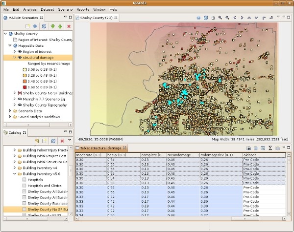
- Now that we can see which buildings in the table have the highest values of mean damage, let's locate those buildings in our map of the area. Make sure the Building Damage layer is still selected in the Scenario View, and make sure you are viewing the 2D Visualization View.
- Then, in the Table View, click on the first row with mean damage Value of highest. You will see one of the dots representing a building in the Visualization View change color to show that this is the selected building.
- Hold shift and click the last row with desired mean damage value. This will select all the buildings in between. You will see these buildings all change color in the Visualization View. This way, you can see which buildings will suffer the most damage. See figure below.
3D Damage Bars
- Now let's add 3d damage bars to the buildings to make it easier to visualize damage across the entire map. Right click the Building Damage layer in the Scenario View, and choose Ranged 3D Visualization...
- Now we can choose which fields we want to display 3d damage bars for. For this example, we will want to see the chance of each damage state, so select Insignific, Moderate, Heavy, and Complete. See figure below
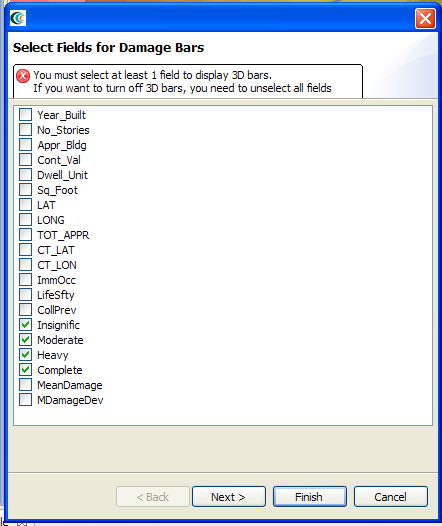
- Click Next. On the next screen, you can choose colors for the various fields. Choose a reasonable set of colors, or use the defaults, then press the Finish button.
- Bring the 3d Visualization View back to the front, and you will see that damage bars have been added for each building. Zoom in and you can quickly see the probable damage states for each building based on the bars. The size of each color in the bar represents the likelihood that the building will be in that damage state. See figure below. Your visualization may differ depending on the fragilities used, whether uncertainty was included in the damage analysis and which hazard was used. In the example below, the Insignific is represented by dark blue, Moderate is represented by light blue, Heavy is represented by green/yellow, and Complete is represented by red.

Aggregating Data
- MAEviz also provides the ability to aggregate data to a geographic boundary, such as the census-tract level. To do this, first add census tract boundary data to your scenario by going to the Catalog view and expanding MAEviz Demo Data -> Boundaries -> Census Tracts, then dragging Shelby County Census Tracts into your Visualization View.
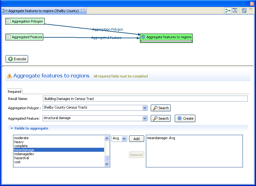
- Now, we want to do an aggregation analysis. Use the Analysis button ( ) again to start the analysis wizard. This time, choose GIS -> Aggregate features to region
- For the Aggregation Polygon field, choose Shelby County Census Tracts. This indicates that you want to aggregate results by the polygon boundaries in the census tract dataset.
- For the Aggregated Feature field, choose your Building Damage dataset. This is where you select which layer contains the data that you want to aggregate over the census tracts.
- For the Result Name field, provide a descriptive name such as Building Damage by Census Tract.
- Last, in the Fields to aggregate section, select the mean damage field in the left text box, select Avg from the drop down menu and click the Add button. You should have something similar to the figure below. Once you are finished adding fields, click the Execute button.
- When the analysis finishes, we need to change the style on the aggregation so that we can easily visualize the results. Right click your new dataset from the Scenario View, and choose Change Layer Style.
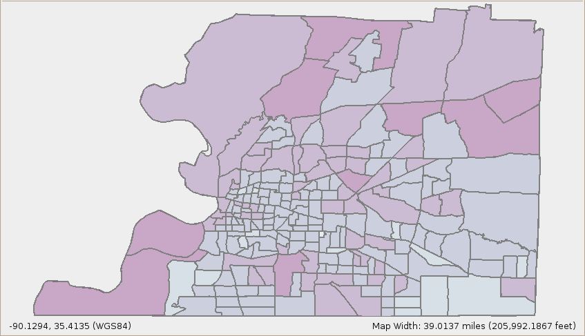
- In the style view, select the Ranged Style tab. Under the Value field, select MeanDamage or any other field you chose to aggregate and want to visualize. If we choose to show MeanDamage, then the census tracts will be colored by the average mean damage value for the buildings in that census tract. Under the color scheme box, select a color scheme that will be easy to see, such as light purple to blue.
Change number of classes to 5, which will give us 5 different shades of color and press the Apply Style button ( ) to apply these style changes. You should see a display similar to the one below.
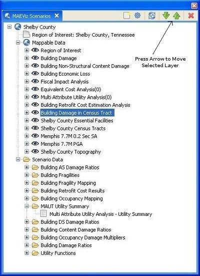
- It will be easier to see the color difference if we select the layer we created (Building Damages in Census Tract) under Mappable Data and press the green up arrow to move the layer up to the top. See figure below.